Topology optimisation of heat conduction problems governed by the Poisson equation
Section author: Patrick E. Farrell <patrick.farrell@maths.ox.ac.uk>
This demo solves example 1 of [3E-GHBS06].
Problem definition
This problem is to minimise the compliance
subject to the Poisson equation with mixed Dirichlet–Neumann conditions
and to the control constraints
where \(\Omega\) is the unit square, \(T\) is the temperature, \(a\) is the control (\(a(x) = 1\) means material, \(a(x) = 0\) means no material), \(f\) is a prescribed source term (here the constant \(10^{-2}\)), \(k(a)\) is the Solid Isotropic Material with Penalisation parameterisation [3E-BendsoeS03] \(\epsilon + (1 - \epsilon) a^p\) with \(\epsilon\) and \(p\) prescribed constants, \(\alpha\) is a regularisation term, and \(V\) is the volume bound on the control.
Physically, the problem is to finding the material distribution \(a(x)\) that minimises the integral of the temperature when the amount of highly conducting material is limited. This code makes several approximations to this physical problem. Instead of solving an integer optimisation problem (at each location, we either have conducting material or we do not), a continuous relaxation is performed; this is standard in topology optimisation [3E-BendsoeS03]. Furthermore, the discrete solution varies as the mesh is refined: the continuous solution exhibits features at all scales, and these must be carefully handled in a discretisation of the problem. In this example we merely add a fixed \(H^1\) regularisation term; a better approach is to add a mesh-dependent Helmholtz filter (see for example [3E-LS11]).
This example demonstrates how to implement general control constraints, and how to use IPOPT [3E-WachterB06] to solve the optimisation problem.
Implementation
First, the dolfin and dolfin_adjoint modules are
imported:
from fenics import *

from fenics_adjoint import *
Next we import the Python interface to IPOPT. If IPOPT is unavailable on your system, we strongly suggest you install it; IPOPT is a well-established open-source optimisation algorithm.
try:
    from pyadjoint import ipopt  # noqa: F401
except ImportError:
    print("""This example depends on IPOPT and Python ipopt bindings. \
  When compiling IPOPT, make sure to link against HSL, as it \
  is a necessity for practical problems.""")
    raise

# turn off redundant output in parallel
parameters["std_out_all_processes"] = False
Next we define some constants, and the Solid Isotropic Material with Penalisation (SIMP) rule.
V = Constant(0.4)  # volume bound on the control
p = Constant(5)  # power used in the solid isotropic material
# with penalisation (SIMP) rule, to encourage the control
# solution to attain either 0 or 1
eps = Constant(1.0e-3)  # epsilon used in the solid isotropic material
alpha = Constant(1.0e-8)  # regularisation coefficient in functional


def k(a):
    """Solid isotropic material with penalisation (SIMP) conductivity
  rule, equation (11)."""
    return eps + (1 - eps) * a ** p
Next we define the mesh (a unit square) and the function spaces to be used for the control \(a\) and forward solution \(T\).
n = 250
mesh = UnitSquareMesh(n, n)
A = FunctionSpace(mesh, "CG", 1)  # function space for control
P = FunctionSpace(mesh, "CG", 1)  # function space for solution
Next we define the forward boundary condition and source term.
class WestNorth(SubDomain):
    """The top and left boundary of the unitsquare, used to enforce the Dirichlet boundary condition."""

    def inside(self, x, on_boundary):
        return (x[0] == 0.0 or x[1] == 1.0) and on_boundary


# the Dirichlet BC; the Neumann BC will be implemented implicitly by
# dropping the surface integral after integration by parts
bc = [DirichletBC(P, 0.0, WestNorth())]
f = interpolate(Constant(1.0e-2), P)  # the volume source term for the PDE
Next we define a function that given a control \(a\) solves the forward PDE for the temperature \(T\). (The advantage of formulating it in this manner is that it makes it easy to conduct Taylor remainder convergence tests.)
def forward(a):
    """Solve the forward problem for a given material distribution a(x)."""
    T = Function(P, name="Temperature")
    v = TestFunction(P)

    F = inner(grad(v), k(a) * grad(T)) * dx - f * v * dx
    solve(F == 0, T, bc, solver_parameters={"newton_solver": {"absolute_tolerance": 1.0e-7,
                                                              "maximum_iterations": 20}})

    return T
Now we define the __main__ section. We define the initial guess
for the control and use it to solve the forward PDE. In order to
ensure feasibility of the initial control guess, we interpolate the
volume bound; this ensures that the integral constraint and the
bound constraint are satisfied.
if __name__ == "__main__":
    a = interpolate(V, A)  # initial guess.
    T = forward(a)  # solve the forward problem once.
With the forward problem solved once, dolfin_adjoint has
built a tape of the forward model; it will use this tape to drive
the optimisation, by repeatedly solving the forward model and the
adjoint model for varying control inputs.
A common task when solving optimisation problems is to implement a callback that gets executed at every functional evaluation. (For example, this might be to record the value of the functional so that it can be plotted as a function of iteration, or to record statistics about the controls suggested by the optimisation algorithm.) The following callback outputs each evaluation to VTK format, for visualisation in paraview. Note that the callback will output each evaluation; this means that it will be called more often than the number of iterations the optimisation algorithm reports, due to line searches. It is also possible to implement callbacks that are executed on every functional derivative calculation.
controls = File("output/control_iterations.pvd")
a_viz = Function(A, name="ControlVisualisation")


def eval_cb(j, a):
    a_viz.assign(a)
    controls << a_viz
Now we define the functional, compliance with a weak regularisation term on the gradient of the material
J = assemble(f * T * dx + alpha * inner(grad(a), grad(a)) * dx)
m = Control(a)
Jhat = ReducedFunctional(J, m, eval_cb_post=eval_cb)
This ReducedFunctional object solves the forward PDE using
dolfin-adjoint’s tape each time the functional is to be evaluated, and
derives and solves the adjoint equation each time the functional
gradient is to be evaluated. The ReducedFunctional object
takes in high-level Dolfin objects (i.e. the input to the evaluation
Jhat(a) would be a dolfin.Function).
Now let us configure the control constraints. The bound constraints are easy:
lb = 0.0
ub = 1.0
The volume constraint involves a little bit more work. Following
[3E-NW06], inequality constraints are represented as
(possibly vector) functions \(g\) defined such that \(g(a)
\ge 0\). The constraint is implemented by subclassing the
InequalityConstraint class. (To implement equality
constraints, see the documentation for
EqualityConstraint.) In this case, our \(g(a) = V -
\int_{\Omega} a\). In order to implement the constraint, we have to
implement three methods: one to compute the constraint value, one to
compute its Jacobian, and one to return the number of components in
the constraint.
class VolumeConstraint(InequalityConstraint):
    """A class that enforces the volume constraint g(a) = V - a*dx >= 0."""

    def __init__(self, V):
        self.V = float(V)
The derivative of the constraint g(x) is constant (it is the diagonal of the lumped mass matrix for the control function space), so let’s assemble it here once. This is also useful in rapidly calculating the integral each time without re-assembling.
    self.smass = assemble(TestFunction(A) * Constant(1) * dx)
    self.tmpvec = Function(A)

def function(self, m):
    from pyadjoint.reduced_functional_numpy import set_local
    set_local(self.tmpvec, m)
Compute the integral of the control over the domain
    integral = self.smass.inner(self.tmpvec.vector())
    if MPI.rank(MPI.comm_world) == 0:
        print("Current control integral: ", integral)
    return [self.V - integral]

def jacobian(self, m):
    return [-self.smass]

def output_workspace(self):
    return [0.0]

def length(self):
    """Return the number of components in the constraint vector (here, one)."""
    return 1
Now that all the ingredients are in place, we can perform the
optimisation. The MinimizationProblem class
represents the optimisation problem to be solved. We instantiate
this and pass it to ipopt to solve:
problem = MinimizationProblem(Jhat, bounds=(lb, ub), constraints=VolumeConstraint(V))

parameters = {"acceptable_tol": 1.0e-3, "maximum_iterations": 100}
solver = IPOPTSolver(problem, parameters=parameters)
a_opt = solver.solve()

File("output/final_solution.pvd") << a_opt
xdmf_filename = XDMFFile(MPI.comm_world, "output/final_solution.xdmf")
xdmf_filename.write(a_opt)
The example code can be found in examples/poisson-topology/ in the
dolfin-adjoint source tree, and executed as follows:
$ mpiexec -n 4 python poisson-topology.py
...
Number of Iterations....: 30

                                 (scaled)                 (unscaled)
Objective...............:   1.3911443093658383e-04    1.3911443093658383e-04
Dual infeasibility......:   5.5344657856725436e-08    5.5344657856725436e-08
Constraint violation....:   0.0000000000000000e+00    0.0000000000000000e+00
Complementarity.........:   3.7713488091294136e-09    3.7713488091294136e-09
Overall NLP error.......:   5.5344657856725436e-08    5.5344657856725436e-08


Number of objective function evaluations             = 31
Number of objective gradient evaluations             = 31
Number of equality constraint evaluations            = 0
Number of inequality constraint evaluations          = 31
Number of equality constraint Jacobian evaluations   = 0
Number of inequality constraint Jacobian evaluations = 31
Number of Lagrangian Hessian evaluations             = 0
Total CPU secs in IPOPT (w/o function evaluations)   =      5.012
Total CPU secs in NLP function evaluations           =     47.108

EXIT: Solved To Acceptable Level.
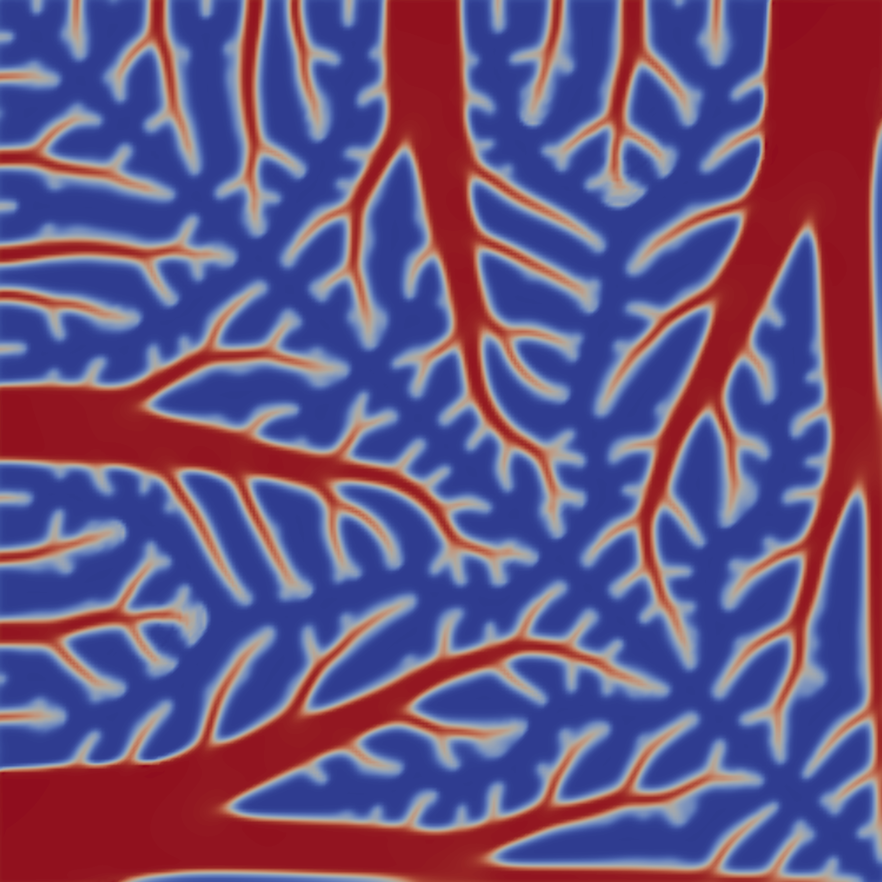
The optimisation iterations can be visualised by opening
output/control_iterations.pvd in paraview. The resulting solution
exhibits fascinating dendritic structures, similar to the reference
solution found in [3E-GHBS06].

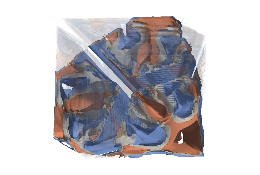
See also examples/poisson-topology/poisson-topology-3d.py for a 3-dimensional
generalisation of this example, with the following solution:

References
M. P. Bendsøe and O. Sigmund. Topology Optimization: Theory, Methods and Applications. Springer, 2003.
A. Gersborg-Hansen, M.P. Bendsøe, and O. Sigmund. Topology optimization of heat conduction problems using the finite volume method. Structural and Multidisciplinary Optimization, 31(4):251–259, 2006. doi:10.1007/s00158-005-0584-3.
B. S. Lazarov and O. Sigmund. Filters in topology optimization based on Helmholtz-type differential equations. International Journal for Numerical Methods in Engineering, 86(6):765–781, 2011. doi:10.1002/nme.3072.
J. Nocedal and S. J Wright. Numerical Optimization. Springer Verlag, 2006.
A. Wächter and L. T. Biegler. On the implementation of an interior-point filter line-search algorithm for large-scale nonlinear programming. Mathematical Programming, 106(1):25–57, 2006. doi:10.1007/s10107-004-0559-y.
